Skip to article frontmatterSkip to article content

Supplementary Material for Chapter 2

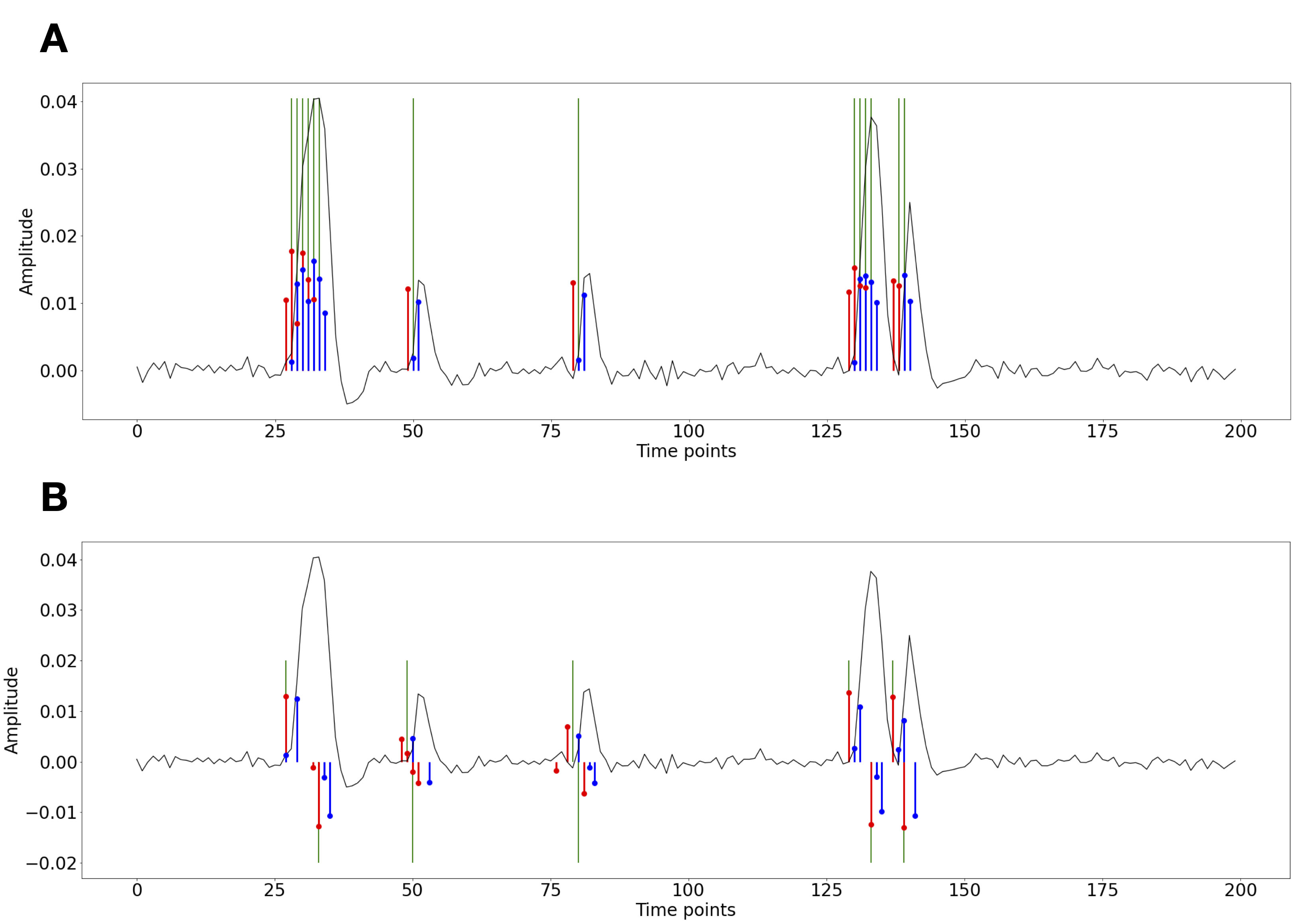
Activity-inducing (A) and innovation (B) signals estimated with
PFM (red) and TA (blue) using their built-in HRF as opposed to using the
same. The black line depicts the simulated signal, while the green lines
indicate the onsets of the simulated neuronal events. X axis shows time
in TRs.

Figure 1:Activity-inducing (A) and innovation (B) signals estimated with PFM (red) and TA (blue) using their built-in HRF as opposed to using the same. The black line depicts the simulated signal, while the green lines indicate the onsets of the simulated neuronal events. X axis shows time in TRs.
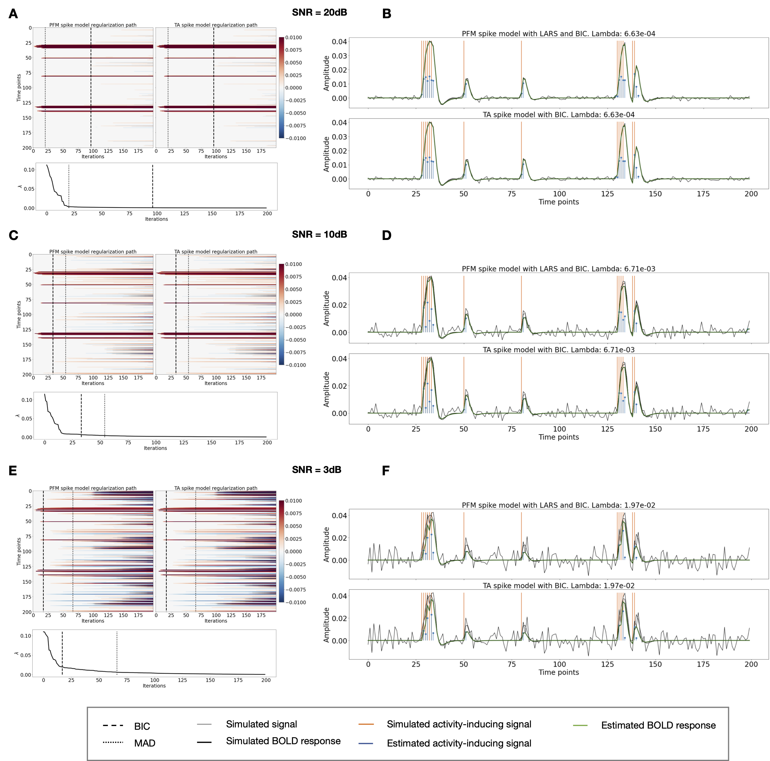
Spike model simulations. (Left) Heatmap of the regularization
paths of the activity-inducing signal estimated with PFM and TA as a
function of \lambda (increasing number of iterations in x-axis),
whereas each row in the y-axis shows one time-point. Vertical lines
denote iterations corresponding to the Akaike and Bayesian Information
Criteria (AIC and BIC) optima. (Right) Estimated activity-inducing (blue)
and activity-related (green) signals when set based on BIC. All estimates
are identical, regardless of SNR.

Figure 2:Spike model simulations. (Left) Heatmap of the regularization paths of the activity-inducing signal estimated with PFM and TA as a function of λ (increasing number of iterations in x-axis), whereas each row in the y-axis shows one time-point. Vertical lines denote iterations corresponding to the Akaike and Bayesian Information Criteria (AIC and BIC) optima. (Right) Estimated activity-inducing (blue) and activity-related (green) signals when set based on BIC. All estimates are identical, regardless of SNR.
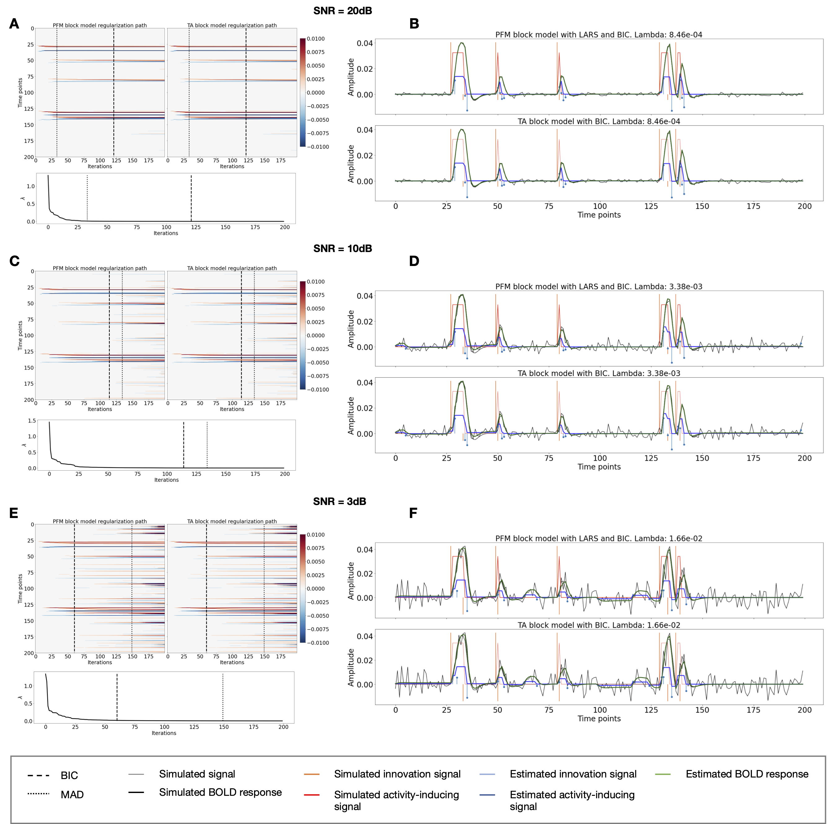
Block model simulations. (Left) Heatmap of the regularization
paths of the innovation signal estimated with PFM and TA as a function
of \lambda (increasing number of iterations in x-axis), whereas
each row in the y-axis illustrates one time-point. Vertical lines denote
iterations corresponding to the Akaike and Bayesian Information Criteria
(AIC and BIC) optima. (Right) Estimated innovation (blue) and
activity-related (green) signals when is set based on BIC. All the
estimates are identical when compared between the PFM and TA cases,
regardless of SNR.

Figure 3:Block model simulations. (Left) Heatmap of the regularization paths of the innovation signal estimated with PFM and TA as a function of λ (increasing number of iterations in x-axis), whereas each row in the y-axis illustrates one time-point. Vertical lines denote iterations corresponding to the Akaike and Bayesian Information Criteria (AIC and BIC) optima. (Right) Estimated innovation (blue) and activity-related (green) signals when is set based on BIC. All the estimates are identical when compared between the PFM and TA cases, regardless of SNR.
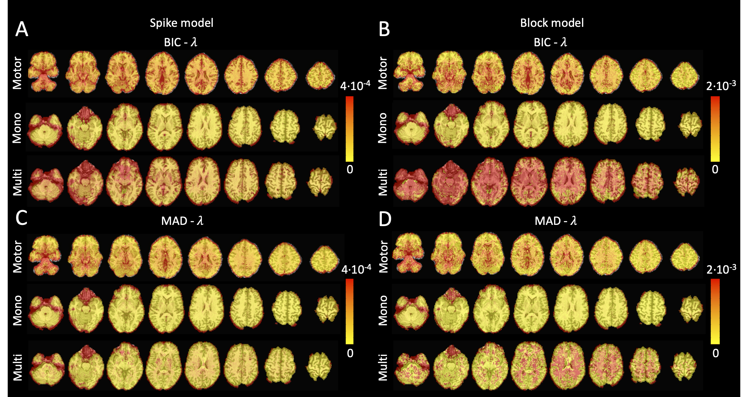
Values of \lambda across the different voxels in the brain
used to estimate (A) the activity-inducing signal (spike model) and (B)
the innovation signal (block model) with the BIC selection, as well as
(C) the activity-inducing signal (block model) and (D) the innovation
signal (block model) with a MAD-based selection. The \lambda maps are
shown for the three experimental fMRI datasets: the motor task (Motor),
the monoband resting-state (Mono), and the multiband resting-state (Multi)
datasets.

Figure 4:Values of λ across the different voxels in the brain used to estimate (A) the activity-inducing signal (spike model) and (B) the innovation signal (block model) with the BIC selection, as well as (C) the activity-inducing signal (block model) and (D) the innovation signal (block model) with a MAD-based selection. The λ maps are shown for the three experimental fMRI datasets: the motor task (Motor), the monoband resting-state (Mono), and the multiband resting-state (Multi) datasets.
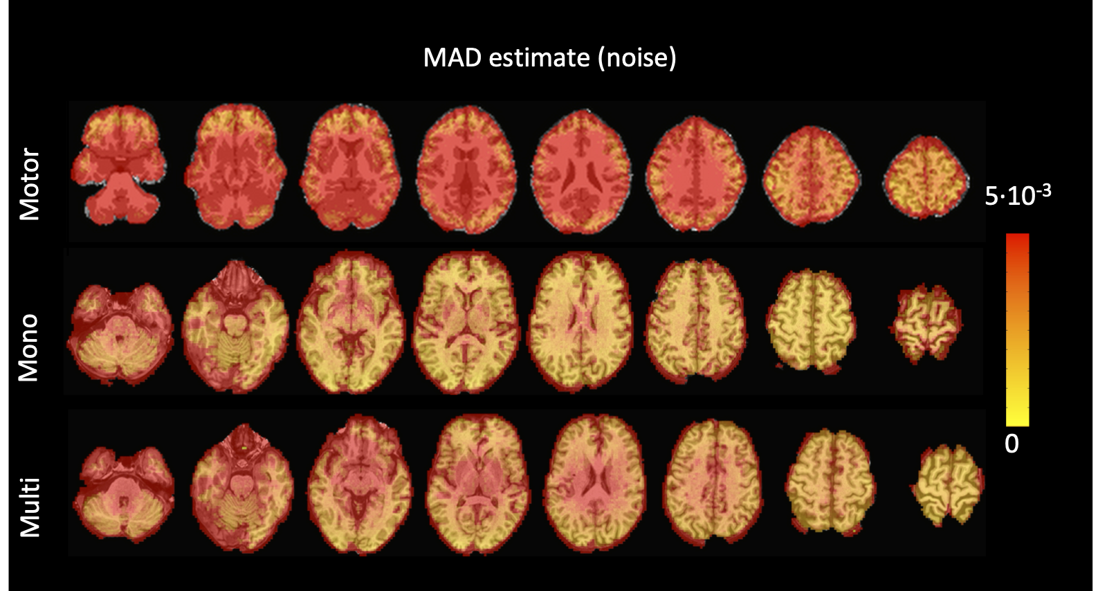
Values of the MAD estimate of standard deviation of the noise
across the different voxels in the brain for the three experimental fMRI
datasets: the motor task (Motor), the monoband resting-state (Mono), and
the multiband resting-state (Multi) datasets.

Figure 5:Values of the MAD estimate of standard deviation of the noise across the different voxels in the brain for the three experimental fMRI datasets: the motor task (Motor), the monoband resting-state (Mono), and the multiband resting-state (Multi) datasets.
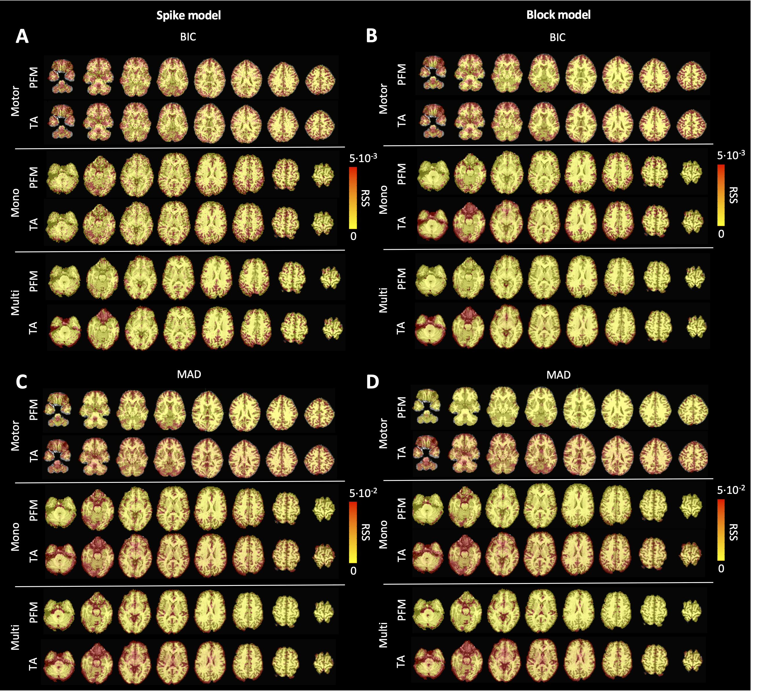
Root sum of squares (RSS) comparison between Paradigm Free Mapping
and Total Activation for the three experimental fMRI datasets: the motor
task (Motor), the monoband resting-state (Mono), and the multiband
resting-state (Multi) datasets. RSS maps are shown for the spike (left) and
block (right) models solved with a selection of \lambda based on the BIC
(top) and MAD (bottom) criteria.

Figure 6:Root sum of squares (RSS) comparison between Paradigm Free Mapping and Total Activation for the three experimental fMRI datasets: the motor task (Motor), the monoband resting-state (Mono), and the multiband resting-state (Multi) datasets. RSS maps are shown for the spike (left) and block (right) models solved with a selection of λ based on the BIC (top) and MAD (bottom) criteria.
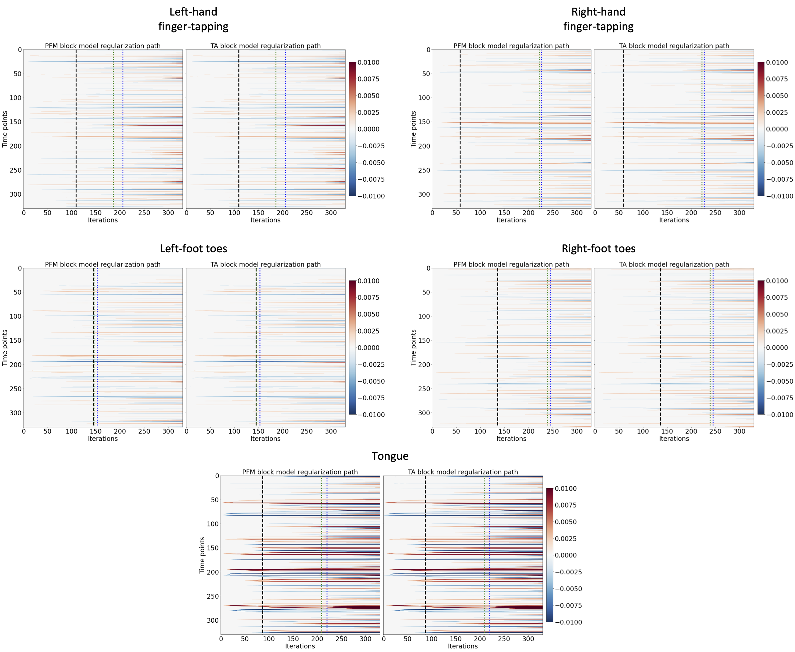
Regularization paths of the innovation signal estimated with
PFM and TA as a function of \lambda (increasing number of iterations in
x-axis, whereas each row in the y-axis shows one time-point) for the
representative voxels of the motor task shown in Figure \cref{fig:task_maps}.
Vertical lines denote selections of \lambda corresponding to the BIC
(black), MAD based on LARS residuals (blue) and MAD based on FISTA residuals
(green) optima.

Figure 7:Regularization paths of the innovation signal estimated with PFM and TA as a function of λ (increasing number of iterations in x-axis, whereas each row in the y-axis shows one time-point) for the representative voxels of the motor task shown in Figure \cref{fig:task_maps}. Vertical lines denote selections of λ corresponding to the BIC (black), MAD based on LARS residuals (blue) and MAD based on FISTA residuals (green) optima.
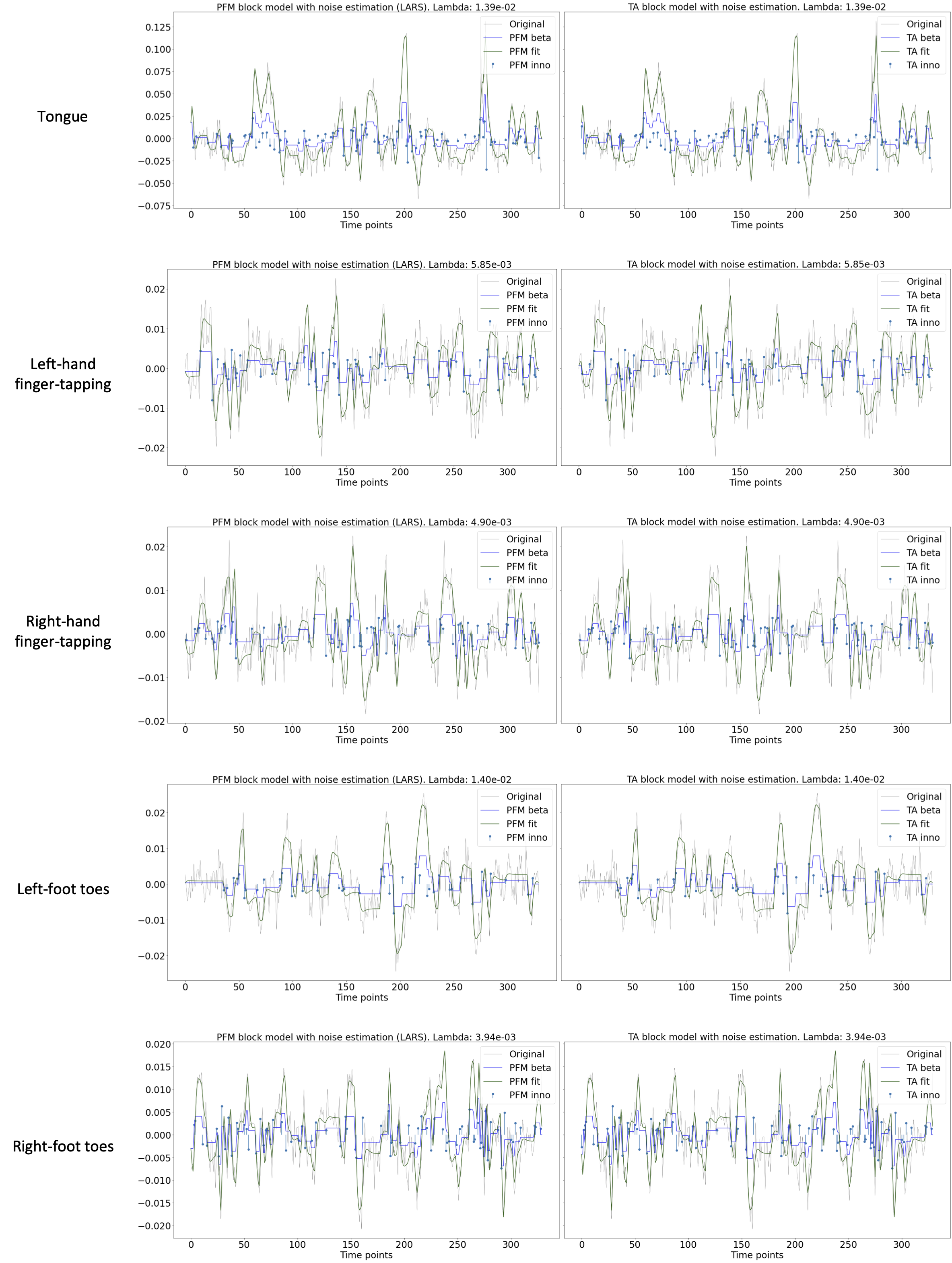
Estimated innovation signal (blue) and activity-related signal
(green) for the representative voxels of the motor task shown in
Figure~\cref{fig:task_maps} with the MAD selection of \lambda made by TA,
i.e., employing the same \lambda with both PFM and TA.

Figure 8:Estimated innovation signal (blue) and activity-related signal (green) for the representative voxels of the motor task shown in Figure~\cref{fig:task_maps} with the MAD selection of λ made by TA, i.e., employing the same λ with both PFM and TA.
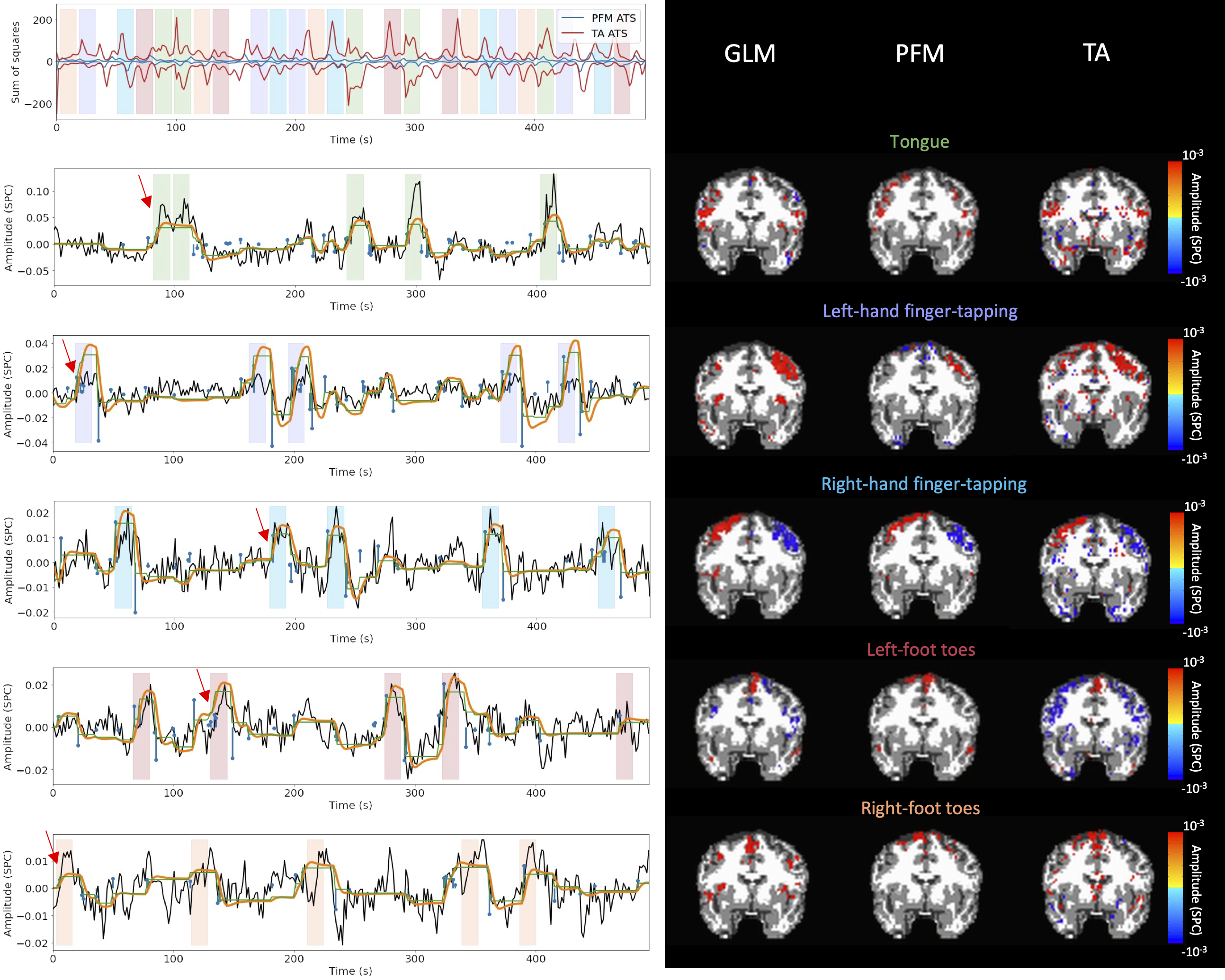
Activity maps of the motor task using a seletion of \lambda based
on the MAD estimate. Row 1: Activation time-series of the innovation signals
estimated by PFM (in blue) or TA (in red) calculated as the sum of squares
of all voxels at every timepoint. Positive-valued and negative-valued
contributions were separated into two distinct time-courses. Color-bands
indicate the onset and duration of each condition in the task (green:
tongue, purple: left-hand finger-tapping, blue: right-hand finger-tapping,
red: left-foot toes, orange: right-foot toes). Rows 2-6: time-series of a
representative voxel for each task with the PFM-estimated innovation (blue),
PFM-estimated activity-inducing (green), and activity-related (i.e., fitted,
orange) signals, with their corresponding GLM, PFM, and TA maps on the
right. The maps shown on the right are sampled at the time-point labeled
with the red arrows and display the innovation signals at that moment across
the whole brain.

Figure 9:Activity maps of the motor task using a seletion of λ based on the MAD estimate. Row 1: Activation time-series of the innovation signals estimated by PFM (in blue) or TA (in red) calculated as the sum of squares of all voxels at every timepoint. Positive-valued and negative-valued contributions were separated into two distinct time-courses. Color-bands indicate the onset and duration of each condition in the task (green: tongue, purple: left-hand finger-tapping, blue: right-hand finger-tapping, red: left-foot toes, orange: right-foot toes). Rows 2-6: time-series of a representative voxel for each task with the PFM-estimated innovation (blue), PFM-estimated activity-inducing (green), and activity-related (i.e., fitted, orange) signals, with their corresponding GLM, PFM, and TA maps on the right. The maps shown on the right are sampled at the time-point labeled with the red arrows and display the innovation signals at that moment across the whole brain.
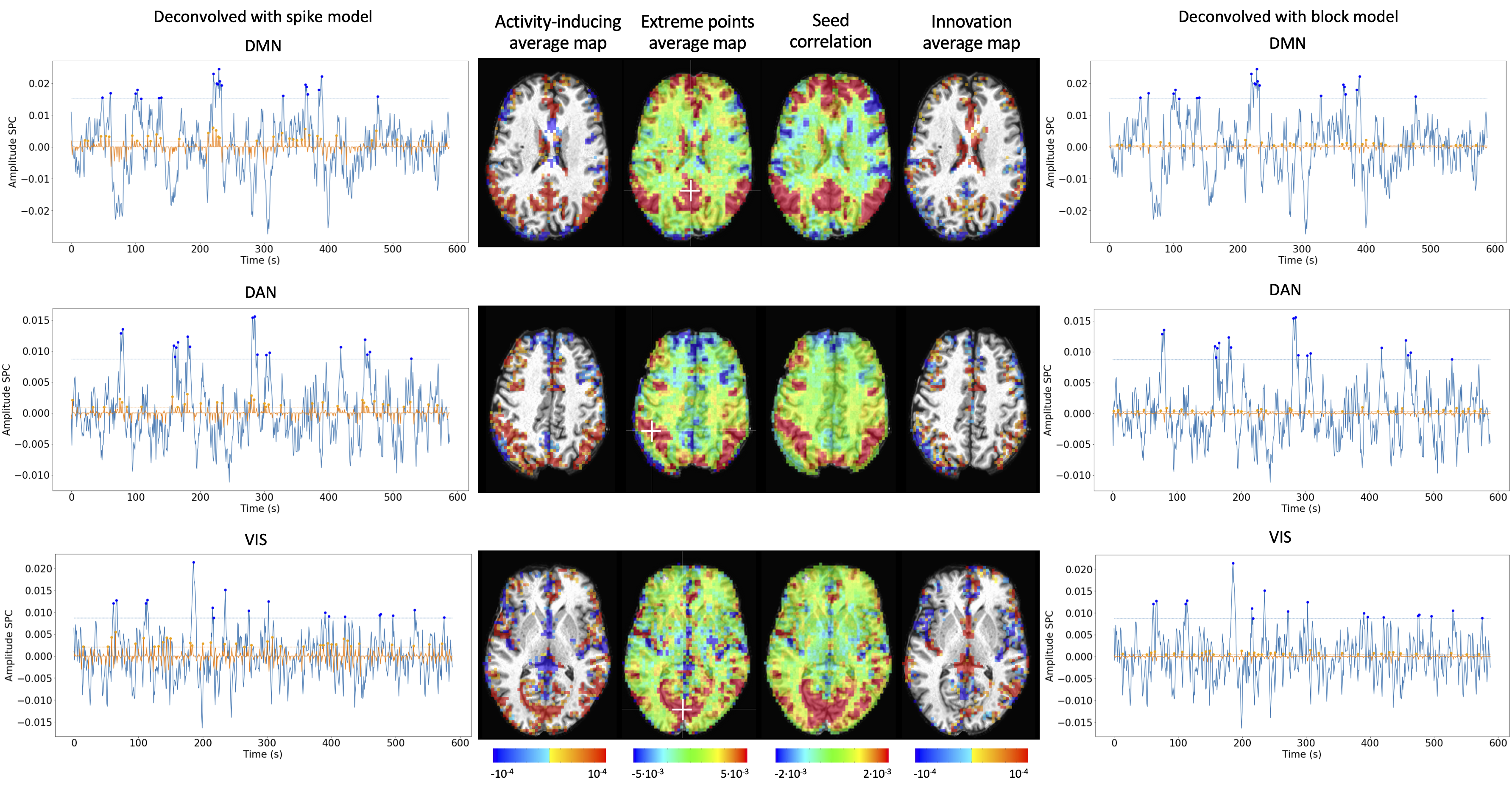
Activity-inducing CAPs (left) and innovation CAPs (right) obtained
with the PFM-estimated activity-inducing and innovation signals
respectively, using a MAD-based selection of \lambda. Time-points selected
with a 95th percentile threshold are shown over the average time-series
(blue) in the seed region (white-cross) and the deconvolved signal (orange).
CAPs and seed correlation maps are illustrated in the center.

Figure 10:Activity-inducing CAPs (left) and innovation CAPs (right) obtained with the PFM-estimated activity-inducing and innovation signals respectively, using a MAD-based selection of λ. Time-points selected with a 95th percentile threshold are shown over the average time-series (blue) in the seed region (white-cross) and the deconvolved signal (orange). CAPs and seed correlation maps are illustrated in the center.