This chapter is in preparation to be published and will be available as an interactive website such as this one.
Functional magnetic resonance imaging (fMRI) during naturalistic paradigms has become increasingly popular in cognitive neuroscience as a way to investigate cognition and behaviour within more ecologically valid contexts. However, current methods for fMRI data analysis in naturalistic paradigms are limited in how they can characterize the precise spatio-temporal dynamics of neural activity evoked by naturalistic stimuli. On the one hand, model-based approaches, such as traditional general linear model (GLM) analyses and encoding models, make strong assumptions about what features of the stimulus might be important and when they occur, which limits an accurate interpretation of the resulting maps of blood oxygenation-level dependent (BOLD) activity. On the other hand, model-free approaches, such as inter-subject correlation and event segmentation algorithms, make no assumptions about stimulus features, but necessitate combining information across multiple time points, making it difficult to trace the recovered signal back to particular moments in the stimulus. To address these limitations, this chapter introduces a novel method for fMRI data analysis in naturalistic paradigms, called multi-subject Paradigm Free Mapping (msPFM). Unlike existing approaches, msPFM estimates shared and individualized neuronal-related brain responses at the finest spatial and temporal resolution available in fMRI data. The msPFM algorithm implements a multivariate regularized least-squares algorithm for hemodynamic deconvolution of fMRI data that estimates the neuronal-related BOLD activity without relying on the temporal structure of the stimuli. Its performance is demonstrated through simulations and experimental movie-watching datasets, showcasing its ability to detect moment-to-moment neuronal-related activity patterns associated with low- and mid-level features of the movie. Furthermore, msPFM reveals a spatial cortical gradient of BOLD activity that aligns with previous findings obtained with event segmentation methods. It also provides an extra temporal dimension to the maps obtained with intersubject correlation analyses. In summary, msPFM offers a powerful tool for exploring the spatio-temporal dynamics of the rich patterns of neural activity evoked by naturalistic fMRI paradigms. Researchers can access the open-source Python package for msPFM at https://github.com/ParadigmFreeMapping/msPFM.
Introduction
The use of movies and stories in the so-called naturalistic paradigms combined with functional magnetic resonance imaging (fMRI) has increased considerably in recent years as a replacement for task and resting state experimental paradigms to study human cognition and mapping brain function Finn, 2021. It owes its popularity not only to its similarity with freeform cognition and unconstrained behaviour, but also to the fact that individual differences in functional connectivity are more stable Vanderwal et al., 2017Wang et al., 2017 and offer improved predictions of behavior Finn & Bandettini, 2021. Furthermore, naturalistic paradigms have emerged as valuable tools for investigating various neurological and developmental disorders. For example, studies utilizing movie-watching have revealed distinct functional network configurations among individuals with autism, highlighting their idiosyncratic patterns Bolton et al., 2018Bolton et al., 2020. Additionally, research has demonstrated a reduction in intersubject correlations within attention-related brain areas among individuals with attention deficit hyperactivity disorder (ADHD), indicating a desynchronization of brain activity in this diseased population Salmi et al., 2020. Movie-watching fMRI has also been utilized to investigate the memory representations of healthy individuals during the retrieval of movie scenes, which revealed a shared spatial organization among subjects exposed to identical naturalistic stimuli Chen et al., 2017. Finally, naturalistic paradigms have played a crucial role in demonstrating the meaningful structure and reliability of movie scene segmentation across subjects Raccah et al., 2022Speer et al., 2009Zacks et al., 2009, }. Notably, studies have revealed that variations in these patterns of event segmentation are associated with age, cognitive abilities Bailey et al., 2017Jafarpour et al., 2022Zacks et al., 2006, and clinical conditions Zalla et al., 2004.
Several techniques have been employed to analyze naturalistic fMRI data. One such technique is intersubject correlation (ISC), which involves calculating the synchrony among the voxelwise signals of multiple subjects throughout the data acquisition process Hasson et al., 2004Wilson et al., 2007Nastase et al., 2019Jangraw et al., 2023Chen et al., 2020. An extension to this approach incorporates the temporal dimension with the sliding window ISC method (averaging ISC over a temporal window of a few volumes) or the instantaneous phase synchronization Glerean et al., 2012, These approaches generate voxelwise measures of moment-to-moment synchrony Nummenmaa et al., 2012, which can then be contrasted against stimulus models, offering an intermediate approach that combines aspects of stimulus-dependent and stimulus-free analyses. However, the degree of synchrony is calculated during the entire acquisition or within the win dow duration, i.e. spanning over multiple TRs. Intra and inter-subject correlation of functional connectivity Vanderwal et al., 2017 and the intersubject correlation of dynamic connectivity Di & Biswal, 2020 offer additional approaches for investigating naturalistic fMRI data that examine the interplay between brain regions and the consistent patterns of connectivity across individuals. Alternatively, the detection of event segmentation boundaries has also been a major focus in the development of data analysis techniques for naturalistic paradigms. Currently, two main state-of-the-art techniques are mostly used to blindly identify temporal boundaries within a sequence of events without prior knowledge: hidden Markov models (HMM) Baldassano et al., 2017 and greedy state boundary search (GSBS) Geerligs et al., 2021. Finally, another strategy involves constructing encoding models that utilize representations extracted from neural network language models to forecast BOLD responses to natural language stimuli Jain et al., 2020, as well as the use of deep neural network models using human visual areas to learn non-hierarchical representations St-Yves et al., 2023.
However, the aforementioned methods have several limitations. First, ISC reveals widespread synchronization across individuals without specific associations with events of particular cognitive functions throughout a scan. Although sliding-window ISC can enhance temporal resolution for characterizing such events, it should be noted that this technique does not offer the utmost level of temporal precision. Second, the HMM and GSBS operate at the ROI level, and hence provide a low spatial resolution that does not allow the discovery of precise, individualized spatial patterns. More importantly, all these techniques summarize the within-region fMRI signal into states or connectivity patterns that are sustained over several TRs, and therefore, they do not capture temporal dynamics at the fastest temporal resolution available in the data, i.e., at the TR level. In summary, these methods rule out the precision mapping of idiosyncratic spatio-temporal patterns evoked by naturalistic stimuli. One possible approach to address this issue is to employ data-driven techniques that operate at the TR and voxel level. Hemodynamic deconvolution is a method that falls under this category Gaudes et al., 2010Karahanoğlu et al., 2013Uruñuela et al., 2023. It has the ability to estimate neuronal-related activity without relying on the temporal information of the experimental paradigm, and as a result, it proves to be particularly valuable when dealing with naturalistic stimuli.
Here, we introduce a novel method for the analysis of naturalistic fMRI data called multi-subject Paradigm Free Mapping (msPFM) that overcomes the limitations mentioned above. msPFM solves a multivariate regularized least-squares problem for hemodynamic deconvolution of the fMRI signal across subjects to blindly estimate the shared and individualized neuronal-related activity without requiring any temporal model of the stimulus. Unlike previous methods for naturalistic fMRI data, this formulation allows the msPFM algorithm to operate at the fastest temporal resolution (TR), and the highest spatial resolution (voxel). We introduce msPFM and evaluate the method in simulations and two experimental datasets with movie-watching paradigms to showcase its potential to elucidate moment-to-moment spatio-temporal neural activity patterns evoked by naturalistic paradigms and assess their ability to map low- and mid-level movie features. The datasets, Iteration and Sherlock, differed in terms of the studied low- and mid-level features, subject counts (43 vs 16), and data type (multi-echo vs single-echo).
Multi-subject Paradigm Free Mapping
Signal Model
In gradient-echo fMRI acquisitions, the time series of a voxel normalized to signal percentage change can be approximated with the following linear relationship with the echo time (TE) Kundu et al., 2017:
where represents BOLD-like changes, describes changes in the net magnetization, and is a random noise term. Changes in the net magnetization are mostly due to motion- and hardware-related artefacts, which can be reduced in preprocessing by using denoising tools such as ICA-AROMA Pruim et al., 2015 for single-echo acquisitions or ME-ICA Kundu et al., 2012Kundu et al., 2017 for multi-echo acquisitions. Hereinafter, the term can be neglected for a simpler notation.
Following the same notation described in previous chapters, let us also consider that changes in that are related to neuronal activity will follow a linear time-invariant model that is defined as the convolution of the activity-inducing signal with the hemodynamic response Boynton et al., 1996Glover, 1999. Considering the signal is sampled at every TR, the previous signal model can be written in discrete matrix form as , where is the Toeplitz convolution matrix with shifted versions of the hemodynamic response function (HRF) Gitelman et al., 2003Gaudes et al., 2013, , , , and is the number of scans (i.e. TRs).
Without loss of generalization, we assume that the HRF model is the same across voxels. As described in Chapter 2: Synthesis-Based and Analysis-Based Hemodynamic Deconvolution for fMRI, the activity-inducing signal can also be written in terms of the innovation signal as , where the matrix is the first-order integration operator Cherkaoui et al., 2019Uruñuela et al., 2020Uruñuela et al., 2023. Hence, the signal model for a given (i.e. single-echo) can be written as follows:
which can be extended for a multi-echo acquisition by concatenating the time series of each echo () in a single vector:
Assuming that data from multiple subjects () are aligned to a common space, the multivariate multi-echo formulation introduced by Uruñuela et al., 2024 (see Chapter 4: Whole-Brain Multivariate Deconvolution for Multi-Echo Functional MRI) is adapted to simultaneously estimate shared and individualized voxelwise activity-inducing signal in multiple subjects. This method, referred to as multi-subject Paradigm Free Mapping (msPFM), therefore proposes to concatenate the voxelwise fMRI signal of multiple subjects into . Hence, for a given voxel or ROI the signal model of msPFM can be written as follows:
which can be simplified as .
Inverse Problem
Assuming the noise follows a Normal distribution, the innovation signals for all subjects can be estimated by solving a multivariate ordinary least squares problem. However, due to high collinearity of the Toeplitz convolution matrix , the estimates will exhibit a large variance in temporal space. Furthermore, in this multi-subject setting where subjects are exposed to the same naturalistic stimuli, certain amount of synchronization of the neuronal activity across subjects can be presumed at given instances. Based on these priors, the estimation of the innovation signal can be solved with the following regularized multivariate least squares problem:
Here, the regularization term promotes sparsity of the innovation signals across time and subjects, treating each estimate independently. On the other hand, the mixed-norm regularization term promotes the co-activation of the innovation signals across all subjects simultaneously Gramfort et al., 2011Uruñuela et al., 2024. The parameter ρ controls the balance between the two regularization terms, and is a diagonal matrix with subject-specific and region-specific regularization parameters , which allows adjusting to the level of noise in each subject’s data and region. Here, the msPFM algorithm is described for multi-echo fMRI data, but note that it can easily be adapted for single-echo data (see Gaudes et al. (2013)).
As it has been discussed in previous chapters, the selection of the regularization parameters is critical to obtain accurate estimates of the innovation signal . Here, for each region, a subject-specific regularization parameter was chosen for each subject , where is a pre-estimated noise level of the data fit and the pre-estimated noise level is derived from the median absolute deviation of fine-scale wavelet coefficients (Daubechies, order 3) of each subject. In addition, the parameter ρ was set to 0.8 to balance the sparsity of the innovation signals (i.e. capturing the idiosyncrasies of each subject and moment) and the grouping of synchronous co-activations across subjects (i.e. shared neuronal responses across subject at a given time). Both the λ and ρ parameters were set based on simulations.
Relevantly, notice that msPFM estimates a 4D dataset of the innovation signal for every subject. That is, unlike a GLM method that calculates activation maps for each onset in the paradigm, msPFM estimates activity maps for each TR. In fact, the innovation signal estimated by msPFM can easily be converted into the activity-inducing signal with an integration operator, and convolved with the HRF to obtain a denoised reconstruction of the data.
Methods
Simulations
We generated a voxel time-series for subjects divided into three groups (groups 1-3) with similar, yet different BOLD patterns to simulate group responses and idiosyncrasies as shown in Figure 1 and Figure 2. We also generated two time-series with no BOLD responses (group 4) as a time-series were msPFM should not find any activity. The time-series included Gaussian noise to simulate the effect of noise in fMRI data, and were normalized to percent signal change.
Two scenarios were simulated to study the effect of how the relative number of subjects in each group affects the estimation of the innovation signal in the other subjects: (1) the groups contained a different ratio of subjects per group: group 1 contained 35 subjects, group 2 contained 15 subjects, and group 3 contained 5 subjects (see Figure 1); and (2) the same ratio of subjects per group is preserved: groups 1, 2 and 3 contain the same amount of subjects (20) as shown in Figure 2.
The data for both scenarios were analyzed with the msPFM algorithm, where for each subject was carefully chosen as , as described in detail in Inverse Problem The parameter ρ was set to 0.8. A Jupyter Notebook with all the simulated scenarios is available at https://github.com/eurunuela/msPFM_paper.
Experimental Data: MR Acquisition and Preprocessing
The performance of the proposed msPFM approach is illustrated in two naturalistic movie-watching datasets acquired with different MRI parameters and with different cognitive characteristics: The Iteration dataset and the Sherlock dataset. These datasets were chosen due to their diffferent characteristics, as they would allow to validate the proposed msPFM method in a broader manner. In particular, Iteration offers 43 subjects and multi-echo data as opposed to Sherlock’s 16 subjects and single-echo data. However, Sherlock has been widely used by the naturalistic fMRI community and thus is well known. In addition, Sherlock contains a higher number of characters compared with the single character in Iteration (a second one appears at the very end), which implies that there is a higher amount of speech present in Sherlock. Finally, the movies are also different in terms of their visuals, with Iteration mostly having a bright background, while Sherlock contains more variety in terms of brightness.
The Iteration Dataset
48 participants were used in this study (all native English speakers; 27F, median age 24.5, range = (19, 64)) from the National Institutes of Health (NIH). See Sava-Segal et al. (2022) for full procedural detail but in brief: subjects watched four movies (ranging from 7:27-12:27 min each) and subsequently completed a task battery designed to probe their interpretations and reactions to the movie, including the following: (i) a 3-min free recall/appraisal task in which subjects spoke freely about their memories and impressions of the movie, during which their speech was captured with a noise-canceling microphone; (ii) multiple-choice comprehension questions designed to ensure they had been paying attention; (iii) multiple-choice and Likert-style items assessing reactions to various characters and to the movie overall. The movie order was pseudorandomized for each subject such that order was counterbalanced at the group level. From the four movies, we selected the one with the clearest event boundaries or scene cuts.
MRI data were collected using a 3T Siemens Prisma scanner with a 64-channel head coil in 43 subjects (all native English speakers; 27F, median age 24.5, range= (19, 64)) while they watched a movie (called Iteration; https://youtu.be/c53fGdK84rc - 12:27 min:sec) at the National Institutes of Health (NIH). All subjects provided informed written consent prior to the start of the study in accordance with experimental procedures approved by the Institutional Review Board of the NIH. Functional images were acquired using a T2*-weighted multiband multi-echo echo-planar imaging (EPI) pulse sequence (TR = 1000 ms, echo times (TE) = [13.6, 31.86, 50.12 ms], flip angle = 60 deg, field of view = 216 x 216 mm, voxel resolution = 3.0 mm isotropic, number of slices = 52 (whole-brain coverage), multiband acceleration factor = 4, with interleaved acquisition). Anatomical images were acquired using a T1-weighted MPRAGE pulse sequence (TR = 2530 ms, TE = 3.30 ms, flip angle = 7 deg, field of view = 256 x 256 mm, voxel resolution = 1.0 mm isotropic). For more details on the data and experimental design, we refer the reader to Sava-Segal et al., 2022. The raw data are available at https://openneuro.org/datasets/ds004516/.
Following the conversion of the original DICOM images to NIFTI format, we used AFNI Cox, 1996 to preprocess MRI data. The preprocessing pipeline was generated with AFNI’s afni_proc function and edited to use tedana The Tedana Community et al., 2022DuPre et al., 2021 for multi-echo independent component analysis (ME-ICA) denoising. Preprocessing included the following steps: despiking, volume realignment, affine coregistration with the subject-specific anatomical T1-weighted image, nonlinear warping to the MNI152_2009 template, multi-echo ICA decomposition with tedana The Tedana Community et al., 2022DuPre et al., 2021, manual classification of ME-ICA components with Rica Uruñuela, 2023, nuisance regression of the components classified as noise, spatial smoothing with an isotropic gaussian kernel with full-width half-maximum of 4 mm, detrending of up to 6th order polynomials, nuisance regression of each subject’s six motion time series, their derivatives, and linear polynomial baselines for each of the functional runs, and normalization to percent signal change. Nuisance regression steps were perfomed together in as single step before normalizing to percent signal change.
Finally, the preprocessed data was then analyzed with a shared response model Chen et al., 2015 in BrainIAK Kumar et al., 2020 to account for different functional topographies across individuals. First, the model was fit to capture reliable whole-brain responses to the movie across subjects in a lower dimensional feature (or component) space of 50 features. Then, the individual voxelwise time courses for each participant were reconstructed using this model. This procedure serves as an additional denoising step and makes spatiotemporal patterns more consistent across subjects. For computational reasons, all analyses were conducted on the average time-series of the 1000 cortical ROIs of the Schaefer atlas Schaefer et al., 2017.
The Sherlock Dataset
16 participants from the Sherlock dataset in Chen et al., 2017 were used for this study. See the original manuscript for full procedural details, but in brief: participants watched a 48-min segment of the BBC television series Sherlock and subsequently verbally recalled the narrative of the show aloud while undergoing fMRI data acquisition. During the recall task participants were instructed to talk for a minimum of 10 minutes, and were allowed to talk for as long as they wished. Experimenters manually ended the scanning run during the recall task based on verbal indication from participants.
MRI data were collected on a 3T Siemens Skyra scanner with a 20-channel head coil. Functional images were acquired using a T2*-weighted echo-planar imaging (EPI) pulse sequence (TR = 1500 ms, TE = 28 ms, flip angle = 64 deg, field of view = 192 × 192 mm\textsuperscript{2}, in-plane resolution = 3.0 × 3.0 mm\textsuperscript{2}, slice thickness = 4 mm, number of slices = 27 (whole-brain coverage) with ascending interleaved acquisition). Reported analyses come from a viewing run of 23 minutes. The raw data were available at https://openneuro.org/datasets/ds001132/versions/1.0.0.
The Sherlock data was preprocessed using fMRIPrep Esteban et al., 2018 with the ICA AROMA option Pruim et al., 2015. The preprocessing also included spatial smoothing with a gaussian kernel of fwhm=6mm, and voxelwise nuisance regression of the 6 realignment parameters, their squares, their derivatives, and squared derivatives. Finally, we performed a detrending step using a 6th order polynomial to remove slow drifts in the data and normalized the data to percent signal change. Similar to The ~Iteration~ dataset, the preprocessed data was then applied the shared response model Chen et al., 2015 in BrainIAK Kumar et al., 2020, and analyses were conducted using the average time-series of the 1000 ROIs from the Schaefer atlas Schaefer et al., 2017.
msPFM and Post Analyses
The msPFM algorithm was employed to estimate the activity-inducing signal for each subject and parcel in the Schaefer 1000-ROI atlas. While msPFM allows for a voxelwise analysis, 1000 ROIs were employed in the analysis for computational efficiency and to address the voxel mismatch issue caused by variations in anatomical structures across subjects. The regularization parameters λ and ρ were selected as described in the simulations section above. The double-gamma SPM HRF was employed via nilearn’s first level GLM module.
Population Synchrony
In order to summarize the estimated activity-inducing signal across subjects and to compute metrics that allow us to validate our method, the positive population synchrony was calculated, denoted as PopSync+. This metric quantifies the number of subjects that show positive neuronal-related activity at each TR, i.e., the number of subjects that activate together in response to the stimuli. This metric was calculated for each ROI, thus obtaining a 4D map of positive population synchrony. Note that unlike other methods that have been used in the literature to quantify population synchrony, this method provides a continuous measure at the TR level, rather than a value per temporal window, which allows us to perform a more fine-grained analysis of the population synchrony.
Event Rate and Inter-Subject Correlation
Recent studies have used hidden Markov model (HMM) algorithms to automatically segment brain activity during the experimental acquisition into a sequence of events (a.k.a. event segmentation). A cortical gradient of segmentation rate has been reported such that primary sensory regions segment (transition between events) more quickly, while higher-order association regions segment more slowly Baldassano et al., 2017Geerligs et al., 2022; this principle has been related to temporal receptive windows and intrinsic timescales of brain regions Murray et al., 2014Hasson et al., 2008. Conversely, these findings suggest a lower occurrence in higher-order association areas that are known to be sensitive to narrative information over longer timescales Lerner et al., 2011Honey et al., 2012. The aim here was to determine if msPFM recovers this same cortical gradient. To this end, the msPFM-based event rate was calculated for each parcel, defined as the number of activity-inducing signal events per minute, using the PopSync+ time series. Only events in the activity-inducing signal that elicited a positive BOLD response were used; i.e., events were defined as instances where the activity-inducing signal remained non-zero for at least 5 TRs.
Another known feature of brain activity during naturalistic stimulation is that synchrony of activity time courses across subjects, known as inter-subject correlation (ISC) Hasson et al., 2004Nastase et al., 2019Finn et al., 2020, also roughly follows a sensory-association gradient, such that subjects are more similar to one another (i.e., more synchronized) in primary visual and auditory regions, while activity becomes more idiosyncratic in higher-order regions. An ISC-like metric was defined from msPFM estimates by quantifying the median correlation across subjects of the estimated activity-inducing signal in each parcel. Then, this was compared to a “classic” ISC approach, in which the median correlation across subjects of average raw BOLD signal was quantified in each parcel.
Correlation Between Population Synchrony and Movie Features
In order to confirm that the multi-subject Paradigm Free Mapping method can detect brain activity
patterns related to sensory stimuli, the correlation between the population synchrony and the
following low-level features was calculated: changes in luminance (i.e., the derivative of the
luminance), and changes in audio (i.e., the derivative of the audio envelope). The low-level
features were extracted from the movies employing a Python package named pliers. More
precisely, the BrightnessExtractor and RMSExtractor functions were used
respectively. The correlation between the population synchrony and the low-level features was
calculated for each ROI, thus obtaining a 3D dataset of correlation values.
The study of the relationship between the brain activity and the naturalistic stimuli was extended
to mid-level features. For instance, naturalistic stimuli where subjects see faces, buildings and
hand-related movements evoke brain activity patterns in the fusiform gyrus
Epstein & Kanwisher, 1998Haxby et al., 2000, the collateral sulcus
Aguirre et al., 1998Epstein & Kanwisher, 1998, and the middle postcentral
sulcus Hasson et al., 2004 respectively. In this study, the primary
focus was to examine the relationship between population synchrony and speech, the presence of
hands, and the presence of faces in the movies. To extract the relevant information, the
ClarifaiAPIVideoExtractor and FaceRecognitionFaceLocationsExtractor functions provided by the
pliers library we utilized. These functions allow to accurately determine the timing of speech
and hand movements, as well as detect the presence of faces in the movie footage.
(sec-multi-subject-results)
Results
Simulations
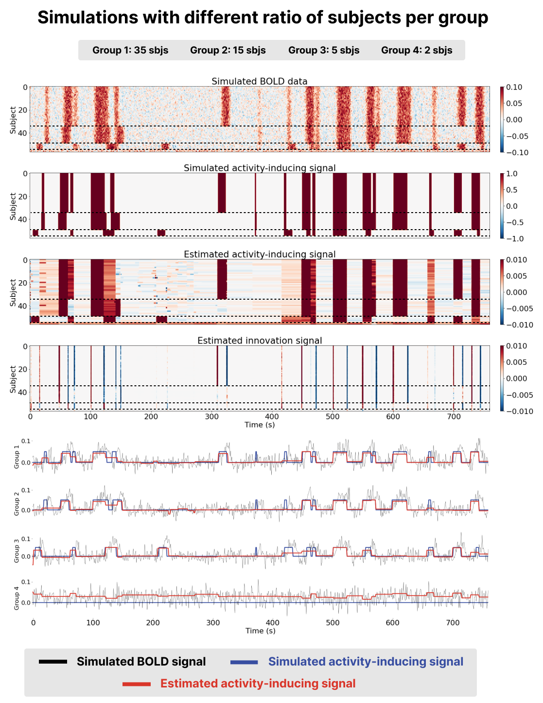
Figure 1:Results of running msPFM on simulated data for a ratio of subjects per group of 35, 15, and 5 subjects respectively (groups are separated by a dashed line). The first two heatmaps represent the simulated BOLD and activity-inducing signals for all the simulated subjects. The third and fourth heatmaps represent the estimated activity-inducing and innovation signals for all the simulated subjects. The time courses below depict the simulated BOLD (black) and activity-inducing (blue) signals for a subject in each group and the estimated activity-inducing signal is shown in red.
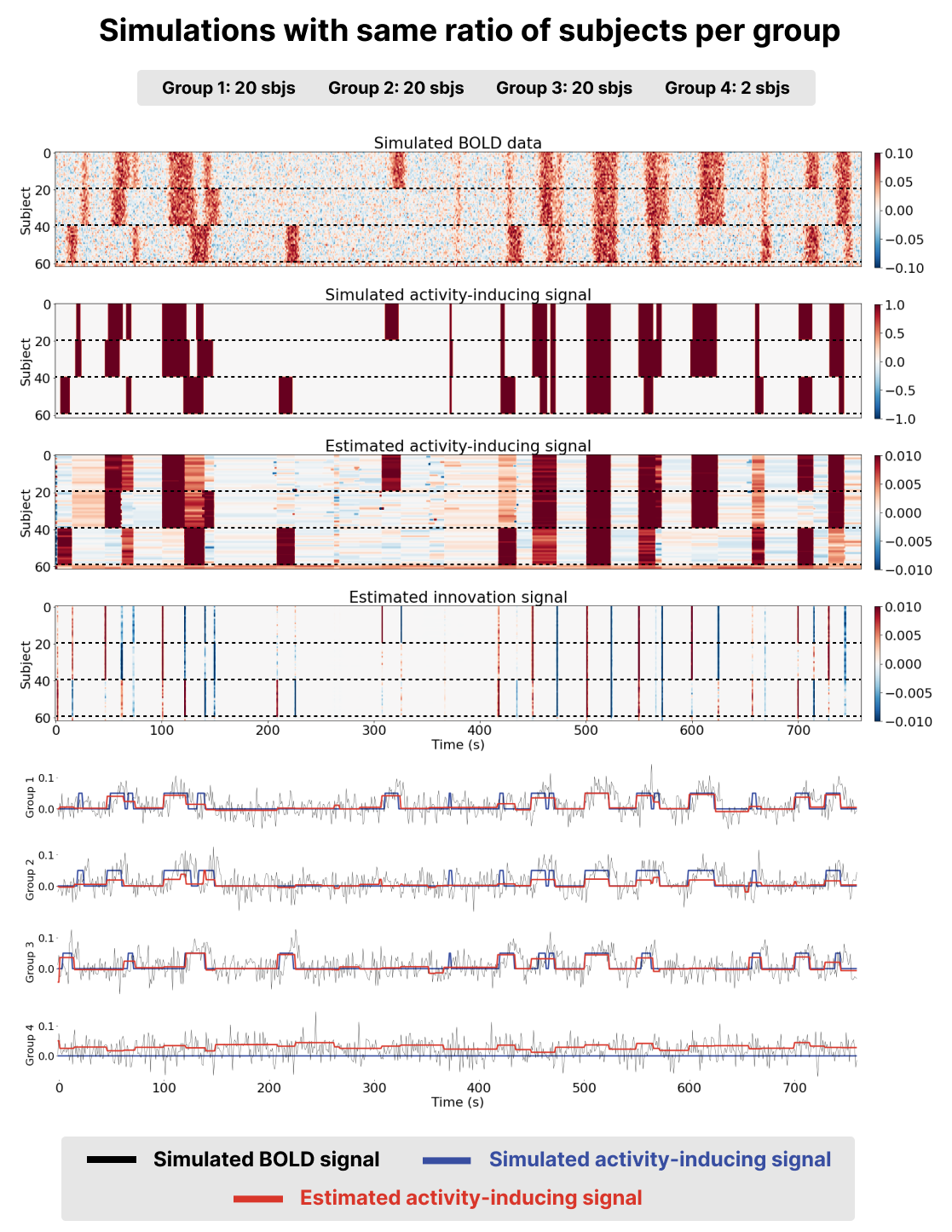
Figure 2:Results of running msPFM on simulated data for a ratio of subjects per group of 20, 20, and 20 subjects respectively (groups are separated by a dashed line). The first two heatmaps represent the simulated BOLD and activity-inducing signals for all the simulated subjects. The third and fourth heatmaps represent the estimated activity-inducing and innovation signals for all the simulated subjects. The time courses below depict the simulated BOLD (black) and activity-inducing (blue) signals for a subject in each group and the estimated activity-inducing signal is shown in red.
Benchmarking msPFM on simulated data where the ground truth is known enables to assess whether it can effectively identify shared neuronal responses across subjects, while accommodating individual differences in response to naturalistic stimuli. The two simulation scenarios described in Methods were employed here.
Visual inspection of the results, as presented in the bottom two heatmaps and the red time courses on Figure 1 and Figure 2, revealed that the activity-inducing signal estimated by msPFM closely resembled the ground truth. This was true for both scenarios, with an unequal and an equal number of subjects per group. msPFM demonstrates proficiency in estimating prolonged activity-inducing signals owing to the adequacy of using a model that estimates the innovations, albeit with relatively lower accuracy in capturing shorter, transient activations (we refer the reader to Uruñuela et al., 2023 for an in-depth comparison between models based on the activity-inducing signal --the spike model-- or the innovations --the block model). Furthermore, the influence of the -norm (see Eq. 5 is conspicuous in the estimation of group four, which lacks simulated activity-signal. In this case, artifacts originating from the estimates of the remaining groups are noticeable, yet these artifacts are relatively minor compared to the estimated activity-inducing signals of the other groups. In addition, the estimated signals for these subjects never return to zero, making it unlikely that they represent any neuronal-related activity and easily identifiable as artefacts. These results are consistent for both scenarios. Hence, based on the simulations, msPFM can pinpoint events that trigger shared and individualized neuronal responses without knowing their timings.
PopSync+ Proof of Concept: Individual and Group Responses to Naturalistic Stimuli
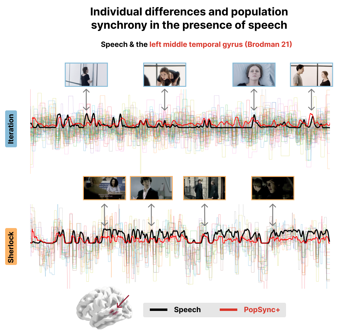
Figure 3:Time series of the estimated activity-inducing signal for each subject in the left middle temporal gyrus (Brodman 21 area) for the Iteration (top) and Sherlock (bottom) datasets. The black lines represent the speech events in the movie. The red lines represent the PopSync+, i.e., the sum across subjects of the activity-inducing signal that evokes a positive BOLD response in each parcel. Representative instances of the movies and their respective Speech and PopSync+ TRs are shown for both datasets.
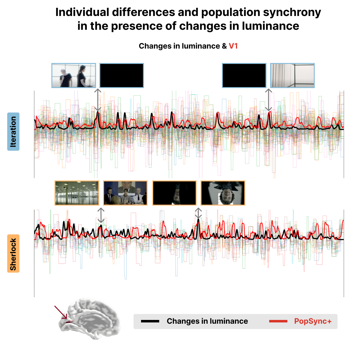
Figure 4:Time series of the estimated activity-inducing signal for each subject in V1 for the Iteration (top) and Sherlock (bottom) datasets. The black lines represent the changes in luminance in the movie. The red lines represent the PopSync+, i.e., the sum across subjects of the activity-inducing signal that evokes a positive BOLD response in each parcel. Representative instances of the movies and their changes in luminance and PopSync+ TRs are shown for both datasets.
Figure 3 and Figure 4 show a proof of concept of the PopSync+ metrics and the individual differences in the estimated activity-inducing signal. In fact, the thinner time series in both datasets clearly demonstrate the presence of individual differences in the msPFM estimates of each subject, ehich are consistly observed in the two examples of the left middle temporal gyrus (Brodman area 21) and the V1 visual area. Notably, the PopSync+ time series (depicted in red) displays a pronounced alignment with speech events occurring in the movies (depicted in black). This alignment is particularly prominent in the context of Sherlock, wherein the episode encompasses a notably higher frequency of speech events compared to Iteration. In the case of the latter, msPFM not only captures the speech events but also identifies additional neural dynamics during non-speech periods in this ROI. Figure 4 illustrates the synchrony between changes in the luminance of the movies and the PopSync+ in V1. Specifically, a stronger alignment is observed in the case of Iteration, where the changes in luminance exhibit greater extremes compared to the case of Sherlock, which is also reflected in the estimated neuronal response in V1 and hence the PopSync+ measure.
Comparison with Hidden Markov Models and Inter-Subject Correlation
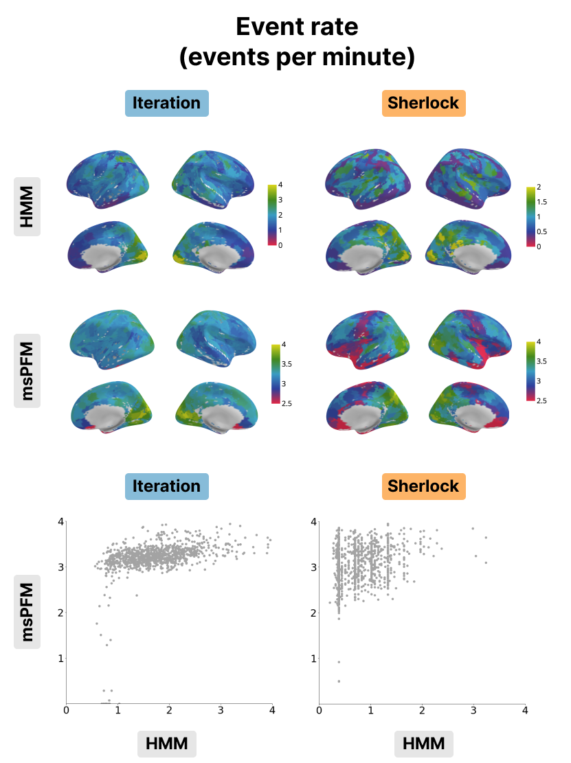
Figure 5:Event rate for the Iteration (left) and Sherlock (right) datasets. The event rate maps obtained with the HMM (top) and msPFM algorithms (bottom) are compared. The bottom row shows the differences in values between msPFM and the HMM approach.
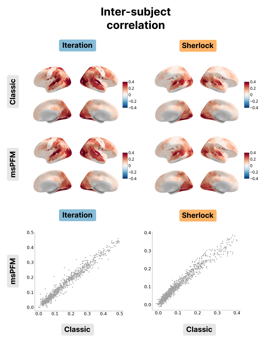
Figure 6:Inter-subject correlation for the Iteration (left) and Sherlock (right) datasets. The inter-subject correlation obtained with msPFM (bottom) is compared with the inter-subject correlation obtained with the classic approach (top). The bottom row shows the differences in values between msPFM and the classical ISC approach.
As shown in Figure 5, the event rates of both HMM and msPFM for the Iteration dataset show a posterior-to-anterior cortical gradient with a higher frequency of events in posterior, sensory regions and slower rates in anterior, higher-order regions. This gradient is consistent with previous findings in the literature Sava-Segal et al., 2022. However, the scatter plots in the bottom row illustrate that the difference in event rates between posterior and anterior regions is less pronounced in the case of msPFM as compared with the HMM. This discrepancy can be attributed to the divergent definitions of what an event is for the two methods. The HMM approach identifies states that are expected to persist for a specific number of time points, while the msPFM algorithm captures “punctate” events that can be directly associated with individual moments in the stimulus. As a consequence, the msPFM algorithm is expected to detect a greater number of events, particularly in anterior regions. In the context of the Sherlock dataset, it is worth noting that the event rate is noticeably lower when calculated with HMM, and consequently, the cortical gradient is less apparent. On the other hand, the msPFM event rate demonstrates values similar to Iteration and reveals a more distinct cortical gradient. When it comes to the inter-subject correlation, the two maps and their values were remarkably similar as shown in Figure 6, indicating that msPFM is able to recover this same sensory-association gradient, with subjects being more synchronized with one another lower-order regions, while being more idiosyncratic in higher-order regions.
Benchmark Against Low- and Mid-Level Movie Features
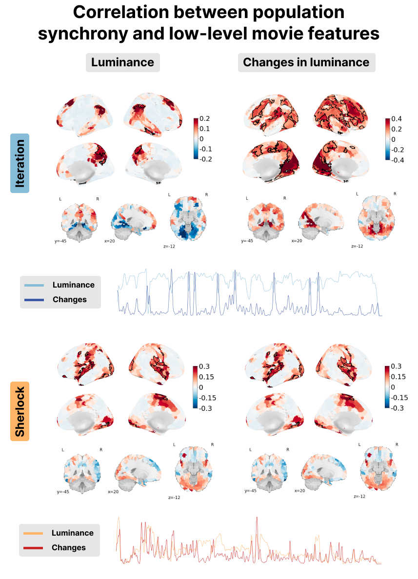
Figure 7:Correlation between the PopSync+ and low-level features of the movie with luminance on the left and its derivative on the right. Significant regions are highlighted by a black contour, while non-significant regions are displayed with increasing transparency as the correlation values are further from the significance threshold. The correlation maps are shown for the Iteration (top) and Sherlock (bottom) datasets. The time courses below depict the luminance (lighter color) and its derivate (darker color) for Iteration (blue) and Sherlock (red).
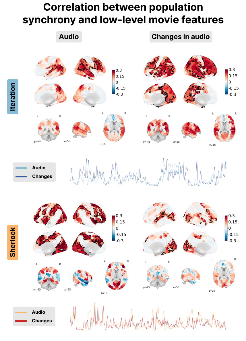
Figure 8:Correlation between the PopSync+ and low-level features of the movie with luminance and its derivative on the left, and the audio envelope and its derivative on the right. Significant regions are highlighted by a black contour, while non-significant regions are displayed with increasing transparency as the correlation values are further from the significance threshold. The correlation maps are shown for the Iteration (top) and Sherlock (bottom) datasets. The time courses of the audio envelope (lighter color) and its derivate (darker color) are shown in blue for Iteration and in red for Sherlock.
The results of the correlation analysis with the low- and mid-level movie features are shown in Figure 7, Figure 8, Figure 9 and Figure 10 respectively.
In terms of luminance, our observations reveal contrasting patterns between Sherlock and Iteration in regions of the visual cortex. While Sherlock demonstrates a positive correlation, indicating a relationship between luminance and brain activity, Iteration exhibits a negative correlation in the same regions. Conversely, when examining changes in luminance (i.e., the derivative of the luminance time course), both datasets display a positive correlation within the visual cortex. These findings can be interpreted as a consequence of the luminance adaptation in Iteration. The movie predominantly features very bright scenes, occasionally transitioning to dark moments as shown in the blue time courses at the bottom left of Figure 7. In contrast, Sherlock contains more diverse scenes in multiple locations, thereby exhibiting a greater range of luminance with both the luminance and its derivative being very similar (see red time courses in the bottom left of Figure 7).
The audio envelope analysis reveals a noteworthy positive correlation within regions of the auditory cortex for both datasets, with a more pronounced correlation observed in Iteration. Examination of audio envelope variations, i.e., the derivate of the audio envelope, further demonstrates a robust positive correlation within the auditory cortex for both datasets. In this case, both the audio envelope and its derivate showed a very similar pattern (see red and blue time courses in the bottom right of Figure 8). This underscores the ability of msPFM to accurately capture the intricate neural dynamics associated with the auditory component of the movies.
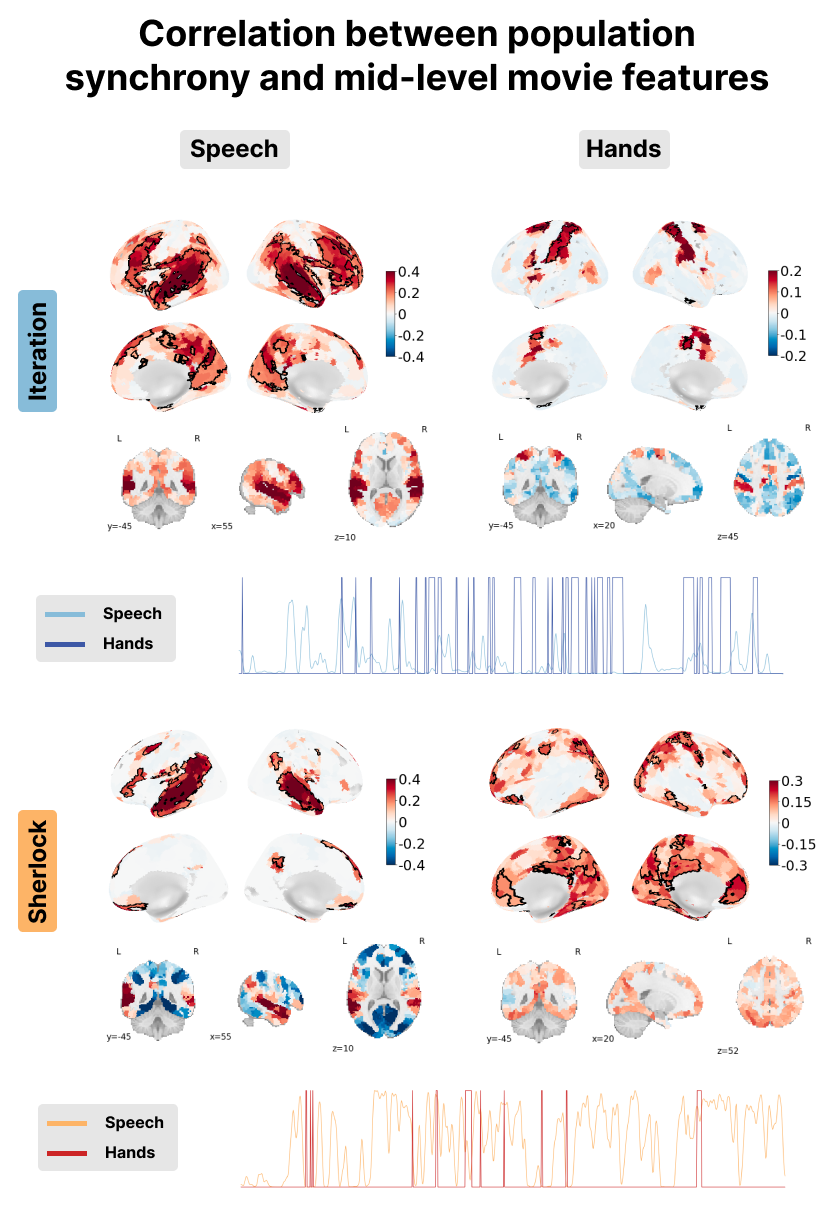
Figure 9:Correlation between the PopSync+ and mid-level features of the movie with the presence of speech on the left and hands on the right. Significant regions are highlighted by a black contour, while non-significant regions are displayed with increasing transparency as the correlation values are further from the significance threshold. The correlation maps are shown for the Iteration (top) and Sherlock (bottom) datasets. The time courses below depict the presence of speech (lighter color) and hands (darker color) for Iteration in blue and Sherlock in red.
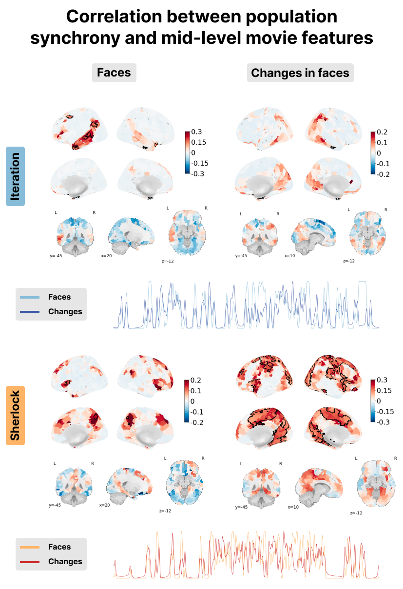
Figure 10:Correlation between the PopSync+ and mid-level features of the movie with the presence of faces on the left and its derivative on the right. Significant regions are highlighted by a black contour, while non-significant regions are displayed with increasing transparency as the correlation values are further from the significance threshold. The correlation maps are shown for the Iteration (top) and Sherlock (bottom) datasets. The time courses of the presence of faces (lighter color) and its derivate (darker color) are shown in blue for Iteration and red for Sherlock.
Next, mid-level movie features were examined, including the presence of speech as well as hands and faces onscreen. Significantly, it can be observed that msPFM adeptly captures the intricate neural dynamics linked to speech in both datasets, revealing large correlations in expected areas of the superior temporal gyrus, Heschl’s gyrus, middle temporal and inferior frontal gyrus, all of them bilaterally. These maps demonstrate the adaptability of msPFM to capture varying amounts of speech present in the respective movies. This adaptability is particularly pronounced in the context of Iteration, characterized by a scarcity of speech compared to Sherlock---a movie abundant in speech- as shown in the time courses in the bottom left of Figure 9. Notwithstanding this discrepancy, msPFM reliably captures the neural dynamics associated with speech in language-related areas, reaffirming its efficacy.
Furthermore, positive correlation between the msPFM-estimated activity-inducing signal and the presence of hands in the movies can also be observed in bilateral sensorimotor regions around the central sulcus. In the context of Iteration, the correlation was observed prominently within regions of the somatosensory cortex (i.e. postcentral gyrus) and supplementary motor areas, while Sherlock exhibited correlation within more anterior regions in the motor cortex (i.e. precentral gyri). These findings could potentially be explained by the contrasting composition of Iteration and Sherlock. While Iteration predominantly incorporates hands in relation to other objects or the main character’s actions (see the high frequency in the blue time course at the bottom left of Figure 9), it features fewer hands-only shots. On the other hand, Sherlock exhibits a higher frequency of hands-only shots (though few across the entire movie as shown in red in the bottom left time course in Figure 9), which may account for the aforementioned findings.
Finally, as shown in Figure 10, correlation between the PopSync+ time-series and the presence of faces was found in the Iteration movie in the left middle temporal gyrus, a region associated with facial familiarity Zhen et al., 2013, and the posterior superior temporal sulcus, a region associated with the processing of gaze and expression Baseler et al., 2012. This finding aligns with the movie’s nature, as Iteration predominantly features a single character and contains several headshots where viewers have their eyes locked on the character’s eyes and can see her facial expression. No significant or substantial correlation between the PopSync+ measure and the presence of faces was found in the movie in the Sherlock dataset. However, when focusing on changes in faces specifically within the Sherlock dataset, a positive correlation was observed in the fusiform gyrus, a region associated with face recognition Kanwisher et al., 1997Kanwisher & Yovel, 2006Rossion et al., 2003 Interestingly, this correlation with changes in faces was not as strong when examining changes in faces for Iteration. These contrasting findings may be attributed to the distinctive characteristics of the movies. In Sherlock, which showcases multiple characters and their facial expressions during dialogue, the adaptation or identification of faces may play a role (see long periods of changing faces in the red time courses at the bottom of Figure 10). On the contrary, Iteration primarily focuses on a single character, suggesting an fMRI adaptation effect in fusiform face areas, i.e. a lower response to an identically repeated face than to new faces Gauthier & Nelson, 2001Yovel & Kanwisher, 2004Avidan & Behrmann, 2010Eger et al., 2005Pourtois et al., 2005Rotshtein et al., 2004.
Overall, these analyses showcase the potential of msPFM in capturing the activity linked to lower- and mid-level stimulus features within anticipated brain regions and timeframes, even without prior knowledge of event timings and regardless of the stimulus itself. Furthermore, these findings highlight the ability of msPFM to identify additional stimulus-specific regions associated with the intricate and distinctive content inherent to each stimulus.
Discussion
The potential of multi-subject Paradigm Free Mapping (msPFM) to detect and elucidate moment-to-moment spatio-temporal neural activity patterns evoked by naturalistic stimuli has been showcased using simulations and two experimental datasets. While previous investigations have employed alternative approaches, such as hidden Markov models (HMM) Baldassano et al., 2017, greedy state boundary search (GSBS) Geerligs et al., 2021, inter-subject correlation Nastase et al., 2019 or dynamic functional connectivity Di & Biswal, 2020, these methods operate on a limited number of regions of interest (ROIs) and condense the temporal dynamics of the BOLD signal into states or connectivity patterns that encompass a time period exceeding the acquired data’s temporal resolution. Consequently, the results shown here highlight the unparalleled potential of msPFM to operate at the utmost temporal and spatial precision achievable.
Importantly, msPFM was validated by comparing it against other common algorithms used to assess naturalistic fMRI data, such as Hidden Markov Models (HMM) and intersubject correlation (ISC). First, the event-rate analysis shown in Figure 5 revealed a distinct cortical gradient, characterized by faster event rates in posterior sensory regions and slower rates in anterior higher-order regions. These results align with previous findings on neural event boundaries across subjects and the segmentation of events using HMM Baldassano et al., 2017Sava-Segal et al., 2022, which could support the idea that the brain’s cortical organization is arranged hierarchically, with sensory inputs passing through unimodal areas and being abstracted into broader conceptual and cognitive representations in transmodal areas Bernhardt et al., 2022Margulies et al., 2016Samara et al., 2023. However, msPFM offers several advantages over the HMM-based approach. First, the HMM method requires specifying a desired number of events () for each region. While there are data-driven ways to estimate an appropriate value for at the group level, these require additional computational time and power, and are not straightforward to implement for individual subjects. In contrast, msPFM does not require pre-specifying any value of , and instead recovers individual neuronal-related events at both the group and individual level. Furthermore, the HMM model assumes that each “state” exhibits a unique neural activity signature that changes at state boundaries, which may not hold true universally, as certain brain regions could potentially revert to previous or new states inside this perdiod. In contrast, msPFM applies no restriction on the number and duration of the neural activity patterns that can be detected, thereby providing a more comprehensive representation of the brain’s spatio-temporal dynamics. The crucial distinction is that the HMM approach identifies events or states that persist for a specific duration, whereas the msPFM technique retrieves discrete instances of neuronal-related BOLD activity, which can be directly associated with individual moments in the stimulus. Another important distinction is the computational cost needed to analyse data with each of the two techniques. In fact, while finding the appropiate number of events with HMM can take h at the single-subject level with 1000 ROIs using a high performance computing server with up to 512GB of RAM available, finding estimates of the activity-inducing signal and counting the number of events with msPFM only took between 5 and 10 minutes.
Furthermore, techniques like HMM and inter-subject correlation are not specifically designed to detect activity evoked by the stimulus in different brain regions, but rather to identify regions that encode stimulus-related information consistently across multiple individuals Nastase et al., 2019. In contrast, msPFM can detect moment-to-moment neuronal resonses not only shared across subject, but also distinguish patterns occurring in individual subjects. By correlating the recovered population synchrony with features of the movies, Figure 7, Figure 8, Figure 9 and Figure 10 show that msPFM is able to detect neuronal activity driven by both low- and mid-level features of the stimulus in both primary sensory and higher-order brain regions. Particularly, fMRI adaptation to the stimulus Grill-Spector & Malach, 2001 may be present in some features such as luminance, with the visual cortex mostly showing activity in response to changes in the luminance in Iteration probably due to the increased contrast associated with these changes Goodyear & Menon, 1998; or the presence of faces, with Iteration having a single character and no reliable face-related activity in the fusiform gyrus as opposed to Sherlock and the many characters in the clip, where the fusiform gyrus showed correlation with changes in faces Kanwisher et al., 1997Kanwisher & Yovel, 2006Rossion et al., 2003. The case of Sherlock is particularly challenging because faces are always closely followed by speech, which is a stronger effect and can hide the response to the presence of faces Vega et al., 2022.
While this study introduces a novel approach for analyzing naturalistic fMRI data, there is potential for further enhancements. Adopting a data-driven strategy like stability selection Meinshausen & Bühlmann, 2010Uruñuela et al., 2024 could eliminate the need for manually selecting the regularization parameter. By adopting such an approach, not only would the method’s robustness be enhanced, but it would also enable estimation of the probability of neuronal-related events at each TR, subject, and voxel or ROI. Additionally, the utilization of optimal transport methods could further refine the spatial differentiation of shared and individualized patterns by improving its robustness against anatomical (spatial) and hemodynamic (temporal) variability between subjects Janati et al., 2020. Nevertheless, the current methodology adequately demonstrates the potential of msPFM-alike approaches in investigating the brain’s spatio-temporal dynamics during naturalistic stimuli. For instance, msPFM offers a valuable approach to unraveling the precise neural mechanisms involved in event segmentation. It can be employed independently or in conjunction with other techniques such as HMM or GSBS to gain an understanding of the timescale for memory encoding, as well as the continuous updating or encoding of memory fragments following the completion of an event Baldassano et al., 2017Silva et al., 2019. Moreover, novel research utilizing msPFM could be aimed at comprehending how the human brain comprehends these complex multiplexed signals and understanding the specific features of the stimulus that elicit responses in the human brain. Finally, the proposed method has the potential to elucidate the connection between individual differences in these responses and subsequent memory formation or appraisal of the stimulus.
Code and data availability
The code and materials used to generate the figures in this work can be found in the following GitHub repository: https://github.com/eurunuela/msPFM_paper.
The msPFM Python package is available in the following GitHub repository: https://github.com/ParadigmFreeMapping/msPFM.
- Finn, E. S. (2021). Is it time to put rest to rest? Trends in Cognitive Sciences, 25(12), 1021–1032. 10.1016/j.tics.2021.09.005
- Vanderwal, T., Eilbott, J., Finn, E. S., Craddock, R. C., Turnbull, A., & Castellanos, F. X. (2017). Individual differences in functional connectivity during naturalistic viewing conditions. NeuroImage, 157, 521–530. 10.1016/j.neuroimage.2017.06.027
- Wang, J., Ren, Y., Hu, X., Nguyen, V. T., Guo, L., Han, J., & Guo, C. C. (2017). Test-retest reliability of functional connectivity networks during naturalistic fMRI paradigms. Human Brain Mapping, 38(4), 2226–2241. 10.1002/hbm.23517
- Finn, E. S., & Bandettini, P. A. (2021). Movie-watching outperforms rest for functional connectivity-based prediction of behavior. NeuroImage, 235, 117963. 10.1016/j.neuroimage.2021.117963
- Bolton, T. A. W., Jochaut, D., Giraud, A.-L., & Ville, D. V. D. (2018). Brain dynamics in ASD during movie-watching show idiosyncratic functional integration and segregation. Human Brain Mapping, 39(6), 2391–2404. 10.1002/hbm.24009